HAIBA and me
Introduction
So. There’s this thing called HAIBA. It is the danish Hospital-Acquired Infections database.
The database is built on the proud danish tradition of databasing everything, it works by crossreferencing the national patient registry (LPR) and the national microbiological database (MiBa). LPR provides times of admission to hospital and transfers between departments. MiBa provides samples taken and sample results from clinical microbiology labs.
The database is great, and it is not so great.
Monitoring hospital-acquired infections is obviously a great goal and the crossreferencing of two massive databases is a gargantuan task. But as a report from the Danish National audit (rigsrevisionen) details, almost no departments actually use the database to improve.
I wanted to analyse differences over time and between departments in the database.
From the database i downloaded 93 datasets - corresponding to one from every department in the region of central Denmark, it took a while. If you want to follow along you can download a csv version of the dataset i made.
library(tidyverse)
library(furrr)
plan(multisession)
library(brms)
library(here)
library(ebbr) #devtools::install_github("dgrtwo/ebbr")
Loading
files <- list.files(here("content", "post", "haiba", "2019-10-21-haiba-and-me", "data_uvi"), recursive = TRUE, full.names = TRUE, pattern = ".csv")

read_haiba <- function(file) {
    blank_lines <- which(grepl("^$", readLines(file)))
    meta <- read_csv(file,
                     skip = blank_lines[length(blank_lines) - 1] - 1,
                     show_col_types = FALSE) %>%
        mutate_all( ~ str_split(.x, ": ") %>% map_chr(2))
    colnames(meta) <- c("sidste_opdatering",
                        "rapport_fra",
                        "region",
                        "ejer",
                        "hospital",
                        "afdeling")
    raw <- read_csv(file,
                    skip = 3,
                    n_max = blank_lines[2] - blank_lines[1] - 2,
                    locale = locale(decimal_mark = ","),
                    show_col_types = FALSE)
    clean <- raw %>%
        select(Year:Denominator2) %>%
        janitor::clean_names() %>%
        rename(week = month) %>%
        mutate(yearweek = sprintf("%i-W%02i", year, week),
               sort_date = paste0(yearweek, "-5") %>% ISOweek::ISOweek2date(),
               date_rank = rank(sort_date)) %>%
        filter(sort_date < lubridate::dmy(meta$sidste_opdatering)[1])
    cbind(clean, select(meta, hospital, afdeling))
}

afd_type <- read_csv("typer.csv", show_col_types = FALSE)
haiba <- future_map_dfr(files, read_haiba) %>%
    left_join(afd_type) %>%
    mutate_at(vars(contains("nominator")), as.integer)
Okay, so that’s loading done. Let’s do some basic checks. It appears that the web-version of HAIBA reports use the columns nominator1 and denominator1.
Exploration
head(haiba)## year week nominator1 incidence1 denominator1 nominator4 incidence3
## 1 2019 4 1 317.04 32 1 317.04
## 2 2019 3 0 0.00 25 0 0.00
## 3 2019 2 0 0.00 15 0 0.00
## 4 2019 1 0 0.00 12 0 0.00
## 5 2018 52 0 0.00 15 0 0.00
## 6 2018 51 0 0.00 13 0 0.00
## denominator2 yearweek sort_date date_rank hospital
## 1 32 2019-W04 2019-01-25 265 Aarhus Universitetshospital
## 2 25 2019-W03 2019-01-18 264 Aarhus Universitetshospital
## 3 15 2019-W02 2019-01-11 263 Aarhus Universitetshospital
## 4 12 2019-W01 2019-01-04 262 Aarhus Universitetshospital
## 5 15 2018-W52 2018-12-28 261 Aarhus Universitetshospital
## 6 13 2018-W51 2018-12-21 260 Aarhus Universitetshospital
## afdeling afd_type
## 1 Akutafdeling Akutafsnit akut
## 2 Akutafdeling Akutafsnit akut
## 3 Akutafdeling Akutafsnit akut
## 4 Akutafdeling Akutafsnit akut
## 5 Akutafdeling Akutafsnit akut
## 6 Akutafdeling Akutafsnit akutmean(haiba$denominator1 < 1) %>% scales::percent()## [1] "16%"with(haiba, mean(nominator1 > denominator1)) %>% scales::percent()## [1] "0%"16% of observations are 0 and some observations seem to show more cases than persondays, which is weird to say the least.
Let’s do a little visualisation
quarters <- data.frame(week = 1:53, quarter = c(rep(1:4, each = 13), 4))

haiba %>%
    left_join(quarters) %>%
    mutate(yearq = paste(year, quarter, sep = "-")) %>%
    group_by(afd_type, yearq) %>%
    summarise(nominator = sum(nominator1),
              denominator = sum(denominator1)) %>%
    ungroup %>%
    filter(denominator > 0) %>%
    mutate(date_rank = dense_rank(yearq)) %>% #Dangerous, but seems to work
    group_by(afd_type) %>%
    group_modify(~ add_ebb_estimate(.x, nominator, denominator)) -> afd_type_quarter
## Joining, by = "week"
## `summarise()` has grouped output by 'afd_type'. You can override using the
## `.groups` argument.## Warning: `data_frame()` was deprecated in tibble 1.1.0.
## Please use `tibble()` instead.
## This warning is displayed once every 8 hours.
## Call `lifecycle::last_lifecycle_warnings()` to see where this warning was generated.ggplot(afd_type_quarter, aes(date_rank, .fitted*1e4, colour = afd_type)) +
geom_smooth(method = "lm", se = FALSE) +
geom_point() +
facet_wrap(~afd_type, scales = "free_y") +
expand_limits(y = 0) +
scale_colour_viridis_d() +
theme(legend.position = "none")## `geom_smooth()` using formula 'y ~ x'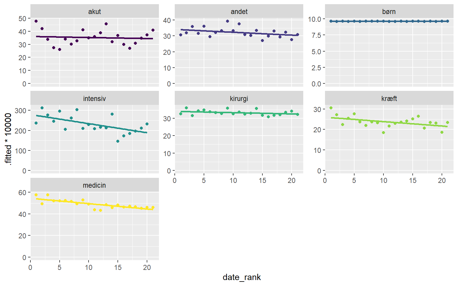
Let’s gussy that up a bit.
ggplot(afd_type_quarter, aes(date_rank, .raw*1e4, colour = afd_type)) +
    geom_ribbon(aes(ymin = .low*1e4, ymax = .high*1e4), fill = "gray", colour = "gray") +
    geom_smooth(method = "lm", se = FALSE) +
    geom_point() +
    facet_wrap(~afd_type, scales = "free_y", labeller = labeller(afd_type = Hmisc::capitalize), nrow = 2) +
    expand_limits(y = 0) +
    scale_colour_viridis_d() +
    scale_x_continuous(breaks = c(seq(0, 20, by = 4))) +
    labs(x = "kvartal fra start",
         y = "incidens pr 10^4 patientdøgn",
         caption = "Data fra HAIBA\n95% Konfidensintervaller baseret på empirical bayes\nLineær regression vist uden konfidensintervaller",
         title = "Hospitalserhvervede urinvejsinfektioner i region midt") +
    theme(legend.position = "none")
## `geom_smooth()` using formula 'y ~ x'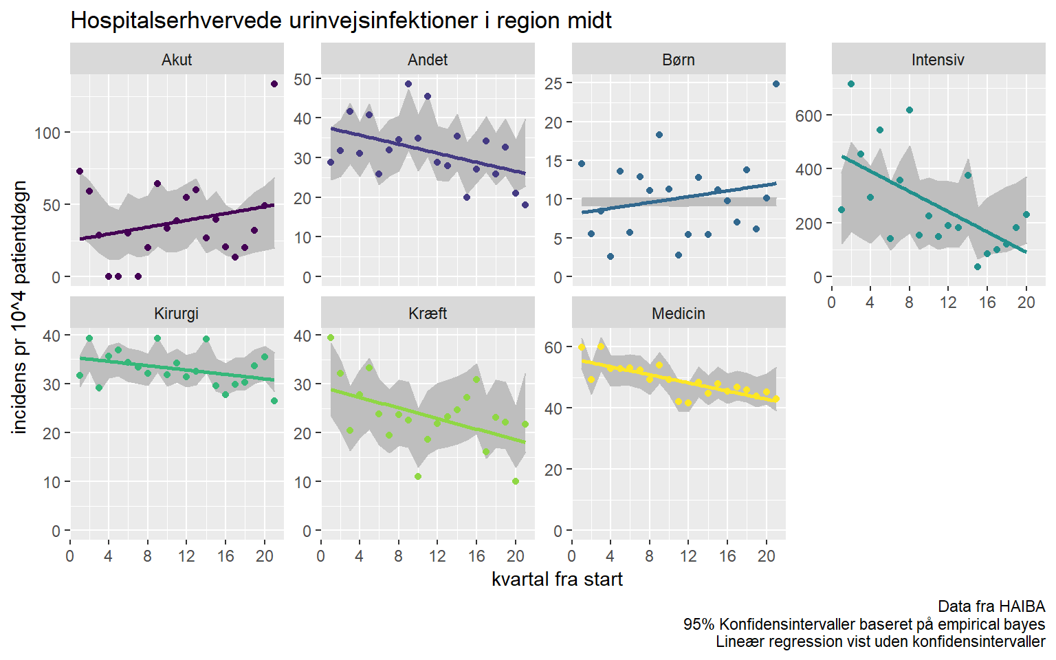
There are some interesting things going on in this visualisation. Most department types seem to be have decreasing UTI incidence. But, what is going on with pediatric and acute departments?
Some insight may be gleaned from the diference between the linear regression on incidence and the grayed out ribbons. Remember, the ribbons display empirical bayes estimates, these are calculated WITHOUT knowledge of the time effects.
For acute departments there appears to be a somewhat seasonal effect, perhaps patients dont stay on the service for long enough to become cases in summer.
Pediatric departments seem more erratic, and it would seem fair to assume that what we’re seeing is merely random variation.
Modeling
If i want an actual answer to whether incidences are decreasing, there’s probably no way around some modeling work.
Seeing as we’re working on count data with large observation times, it would seem reasonable to model the outcome as poisson distributed.
I want to be able to compare individual departments on their initial incidence, their progress over time, and their incidence at the end. I could feasibly fit a normal glm model with offset = log(denominator1) and fixed effects for departments, but some departments are much smaller than others and their mere size would bias the analysis so that large departments would look closer to average, just from having less random variation.
So, what i actually want is a bayesian model with partial pooling on departments for both intercept and slope, fixed effects for department type. Let’s see if i can figure that out
halfyear <- data.frame(week = 1:53, halfyear = c(rep(1:2, each = 26), 2))

null_departments <- haiba %>% # Some departments have 0 cases in total. Thats great, but not very informative.
    group_by(afdeling) %>%
    summarise(nominator = sum(nominator1),
              denominator = sum(denominator1)) %>%
    filter(nominator == 0)

haiba %>%
    anti_join(null_departments, by = "afdeling") %>% # Potentielt kontroversielt, men i praksis nok mere data-cleaning
    left_join(halfyear) %>%
    mutate(yearh = paste(year, halfyear, sep = "-")) %>%
    group_by(afdeling, yearh) %>%
    summarise(nominator = sum(nominator1),
              denominator = sum(denominator1),
              afd_type = unique(afd_type)) %>%
    ungroup %>%
    filter(denominator > 0) %>%
    mutate(date_rank = dense_rank(yearh)) -> afdeling_halfyear
## Joining, by = "week"
## `summarise()` has grouped output by 'afdeling'. You can override using the
## `.groups` argument.mm_data_afd <- afdeling_halfyear %>%
mutate_at(vars(contains("nominator")), as.integer) %>%
mutate_at(vars(contains("afd")), as.factor)brms model
n_cores <- parallel::detectCores()
model <- brm(nominator ~ 0 + offset(log(denominator)) + date_rank + afd_type + (1 + date_rank | afdeling),
          data = mm_data_afd,
          family = "poisson",
          chains = n_cores, cores = n_cores, file = here("content", "post", "haiba", "2019-10-21-haiba-and-me", "model"))
Model checks
Did the chains converge?
plot(model)
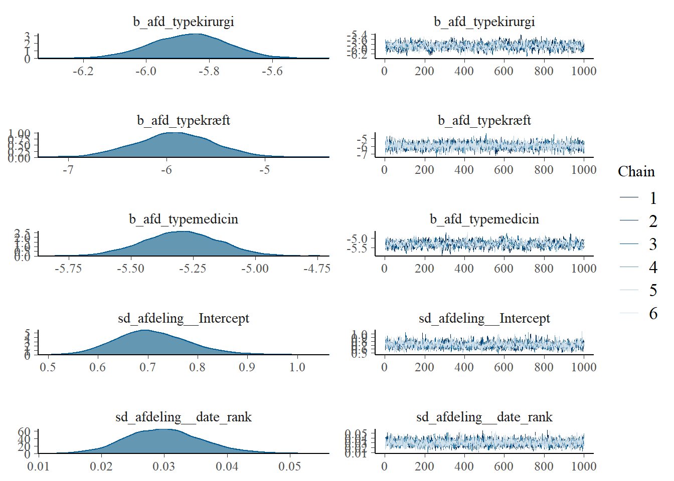

Seems reasonable enough.
model## Family: poisson
## Links: mu = log
## Formula: nominator ~ 0 + offset(log(denominator)) + date_rank + afd_type + (1 + date_rank | afdeling)
## Data: mm_data_afd (Number of observations: 822)
## Draws: 6 chains, each with iter = 2000; warmup = 1000; thin = 1;
## total post-warmup draws = 6000
##
## Group-Level Effects:
## ~afdeling (Number of levels: 80)
## Estimate Est.Error l-95% CI u-95% CI Rhat Bulk_ESS
## sd(Intercept) 0.71 0.07 0.58 0.87 1.01 1420
## sd(date_rank) 0.03 0.01 0.02 0.04 1.00 2150
## cor(Intercept,date_rank) -0.41 0.19 -0.73 0.02 1.00 2630
## Tail_ESS
## sd(Intercept) 2875
## sd(date_rank) 3391
## cor(Intercept,date_rank) 4044
##
## Population-Level Effects:
## Estimate Est.Error l-95% CI u-95% CI Rhat Bulk_ESS Tail_ESS
## date_rank -0.02 0.01 -0.03 -0.01 1.00 2836 3828
## afd_typeakut -5.54 0.33 -6.20 -4.88 1.00 3854 4202
## afd_typeandet -5.88 0.24 -6.35 -5.41 1.00 1969 2427
## afd_typebørn -6.88 0.38 -7.62 -6.15 1.00 3958 4450
## afd_typeintensiv -3.88 0.69 -5.22 -2.49 1.00 5174 4229
## afd_typekirurgi -5.86 0.12 -6.11 -5.63 1.00 1017 1925
## afd_typekræft -5.92 0.40 -6.70 -5.16 1.00 2634 3600
## afd_typemedicin -5.30 0.15 -5.59 -5.01 1.00 803 1294
##
## Draws were sampled using sampling(NUTS). For each parameter, Bulk_ESS
## and Tail_ESS are effective sample size measures, and Rhat is the potential
## scale reduction factor on split chains (at convergence, Rhat = 1).No dire warnings here either. Effective sample sizes could be higher.
Hypothesis 1: Infection control is improving
Lets test the hypothesis that number of cases is falling over time
hypothesis(model, "date_rank < 0")## Hypothesis Tests for class b:
## Hypothesis Estimate Est.Error CI.Lower CI.Upper Evid.Ratio Post.Prob
## 1 (date_rank) < 0 -0.02 0.01 -0.03 -0.01 299 1
## Star
## 1 *
## ---
## 'CI': 90%-CI for one-sided and 95%-CI for two-sided hypotheses.
## '*': For one-sided hypotheses, the posterior probability exceeds 95%;
## for two-sided hypotheses, the value tested against lies outside the 95%-CI.
## Posterior probabilities of point hypotheses assume equal prior probabilities.marginal_effects(model, "date_rank", spaghetti = TRUE, nsamples = 1e3, conditions = data.frame(denominator = 1e4))## Warning: Method 'marginal_effects' is deprecated. Please use
## 'conditional_effects' instead.## Warning: Argument 'nsamples' is deprecated. Please use argument 'ndraws'
## instead.
It would appear beyond reasonable doubt that there is indeed a falling incidence of HA-UTI. What is the magnitude of this fall?
broom.mixed::tidy(model) %>%
  filter(term == "date_rank") %>%
  select(-std.error) %>%
  mutate_at(vars(estimate:conf.high), ~ 1 - exp(. * (mm_data_afd$date_rank %>% range %>% diff))) %>%
  mutate_at(vars(estimate:conf.high), scales::percent) %>%
  glue::glue_data("The overall reduction from the beginning of HAIBA (2014 week 1) to the latest point in our dataset (2019 week 4) is {estimate} [95% CI: {conf.high}; {conf.low}]")
## Warning in tidy.brmsfit(model): some parameter names contain underscores: term
## naming may be unreliable!## The overall reduction from the beginning of HAIBA (2014 week 1) to the latest point in our dataset (2019 week 4) is 16% [95% CI: 5%; 25%]Are any departments falling way out of line with the overall trend?
hypothesis(model, "date_rank = 0", group = "afdeling", scope = "ranef") %>%
  .$hypothesis %>%
  filter(Star == "*") -> differently_changed

mm_data_afd %>%
    semi_join(differently_changed, by = c("afdeling" = "Group")) %>%
    ggplot(aes(date_rank, nominator/(denominator/1e4), colour = afdeling)) +
    geom_point() +
    scale_colour_viridis_d(option = "A") +
    geom_smooth(method = "lm", se = FALSE) +
    expand_limits(y = 0)
## `geom_smooth()` using formula 'y ~ x'
It would appear that both departments have made massive improvements.
Hypothesis 2: Departments are (very) different
conditional_effects(model, "afd_type", conditions = data.frame(denominator = 1e4))
last_plot() + coord_flip()
Okay, so intensive care units have more cases. That’s probably not a big surprise to anyone. Many of the “cases” are probably misclassifications due to more frequent urinary sampling and the increased difficulty in ascertaining symptoms from patients in intensive care.
hypothesis(model, "Intercept = 0", group = "afdeling", scope = "ranef") %>%
    .$hypothesis %>%
    filter(Star == "*") -> differently_started

differently_started %>%
    mutate(Group = forcats::fct_reorder(Group, Estimate)) %>%
    ggplot(aes(Group, exp(Estimate), colour = Estimate)) +
    geom_ribbon(aes(ymin = exp(CI.Lower), ymax = exp(CI.Upper))) +
    geom_point() +
    scale_colour_viridis_c(option = "C") +
    theme(legend.position = "none") +
    coord_flip() +
    labs(y = "Rate ratio ifht afdelingstype", x = NULL,
caption = "Data fra HAIBA\nVist med 95% konfidensintervaller") 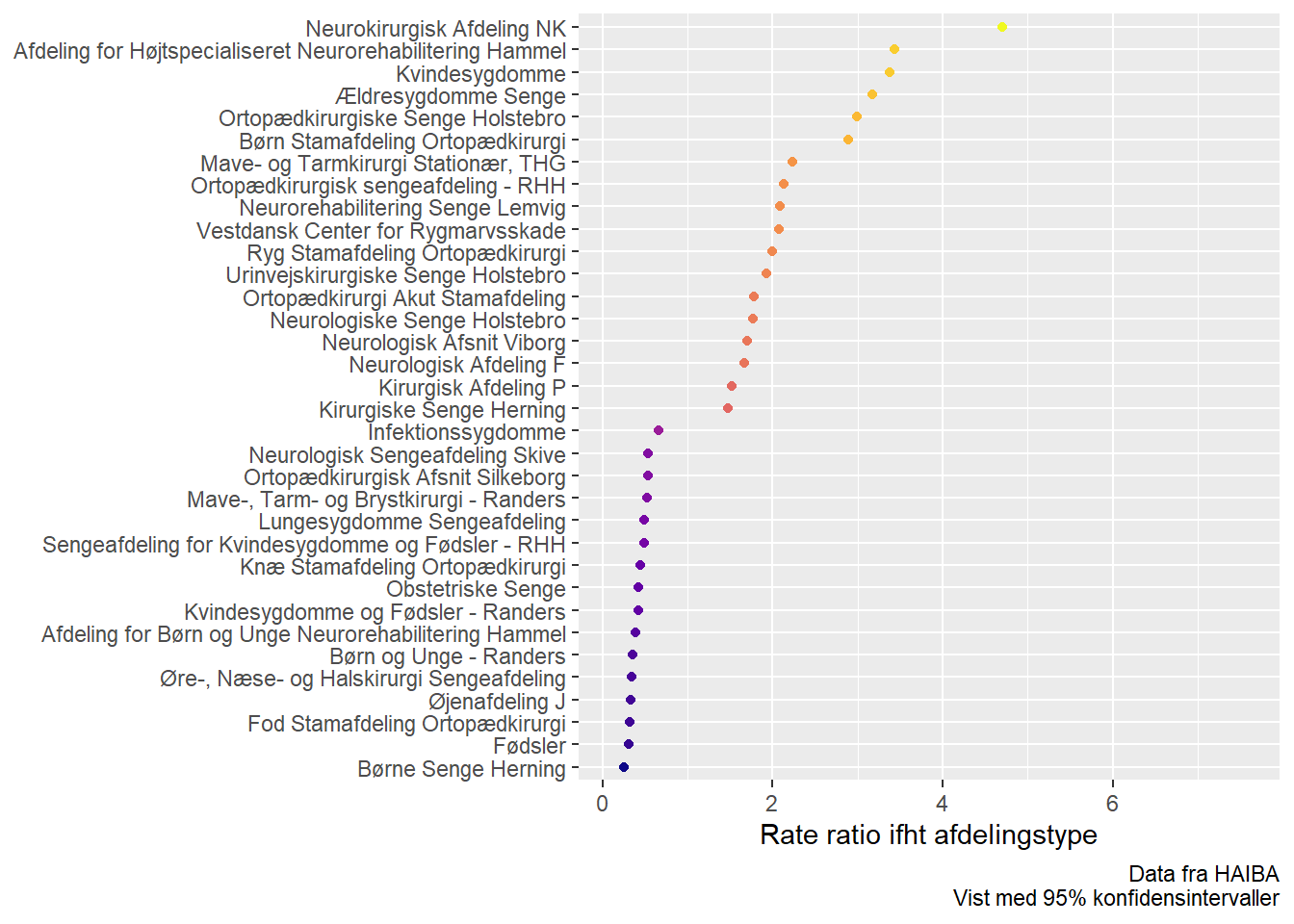
A few surprises here, but overall as expected. Some of the departments seem to have been picked up due to insufficient correction in the “Other” department type.
That’s the intercept done with. But where do these departments end up? Do they come into line with the pack?
new_from_differently_started <- mm_data_afd %>%
  semi_join(differently_started, by = c("afdeling" = "Group")) %>%
  select(afdeling, afd_type) %>%
  distinct() %>%
  mutate(date_rank = 12,
         denominator = 1e4)

quick_clean <- . %>%
  as_tibble() %>%
  janitor::clean_names()

predictions <- predict(model, newdata = new_from_differently_started) %>%
  quick_clean %>%
  bind_cols(new_from_differently_started) %>%
  mutate(condition = "At end")

unknown_departments <- mm_data_afd %>%
  distinct(afd_type) %>%
  mutate(afdeling = wakefield::name(n()),
         date_rank = 12,
         denominator = 1e4)

predicted_beginnings <- predict(model, newdata = new_from_differently_started %>% mutate(date_rank = 1)) %>%
  quick_clean() %>%
  bind_cols(new_from_differently_started %>% select(afdeling)) %>%
  mutate(condition = "At beginning")

predictions_for_unknown <- predict(model, newdata = unknown_departments, allow_new_levels = TRUE) %>%
  as_tibble() %>%
  janitor::clean_names() %>%
  bind_cols(unknown_departments) %>%
  mutate(condition = "Unknown department")

different_started_by_the_end <- predictions %>%
  left_join(predictions_for_unknown, by = "afd_type") %>%
  left_join(predicted_beginnings, by = c("afdeling.x" = "afdeling"), suffix = c("", ".z"))

bind_rows(predicted_beginnings, predictions) %>%
  left_join(predictions_for_unknown, by = "afd_type", suffix = c("", ".y")) %>%
  mutate(afdeling = forcats::fct_reorder(afdeling, estimate, .fun = first)) %>%
  ggplot(aes(afdeling, estimate, colour = condition)) +
  geom_ribbon(aes(afdeling, ymin = q2_5, ymax = q97_5), data = ~ filter(.x, condition == "At end"), colour = "gray") +
  geom_point() +
  geom_point(aes(afdeling, estimate.y, colour = "Department type"), show.legend = TRUE) +
  coord_flip() +
  scale_colour_brewer(palette = "Set2", direction = -1) +
  theme(legend.position = "bottom") +
  labs(x = "Department",
       y = "Cases pr. 10000 persondays",
       colour = "Prediction case",
       caption = "Data from HAIBA")
## Warning: Removed 34 rows containing missing values (geom_point).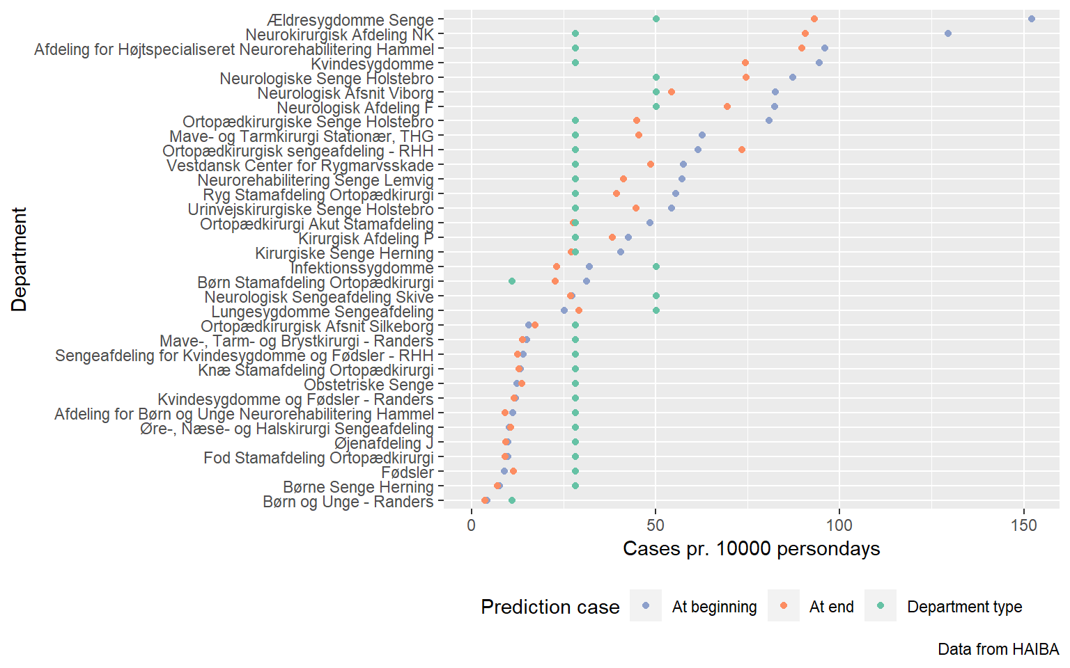
Honorable mention to the departments without any cases
null_departments %>% arrange(desc(denominator))## # A tibble: 13 × 3
## afdeling nominator denominator
## <chr> <int> <int>
## 1 Livsstilscenter Brædstrup, Sengeafdeling - BRÆ 0 31597
## 2 Fokuseret Neurorehabilitering Hammel 0 13759
## 3 Tand-, Mund- og Kæbekirurgi Sengeafdeling 0 2493
## 4 Hånd Stamafdeling Ortopædkirurgi 0 2475
## 5 Skulder Stamafdeling Ortopædkirurgi 0 1677
## 6 Idræt Stamafdeling Ortopædkirurgi 0 1220
## 7 Brystkirurgi Stationær 0 678
## 8 Øre-, Næse- og Halssygdomme - Randers 0 290
## 9 Infektion Stamafdeling Ortopædkirurgi 0 28
## 10 Akutmodtagelse Q - Randers 0 21
## 11 Øjenafdeling Dagkirurgi Stationær J 0 16
## 12 Neurokirurgisk Dagkirurgi Stationær NK 0 15
## 13 Kirurgisk Dagkirurgi P Stationær Afdeling 0 6